10 Tips to be the Smartest User on Google Spreadsheets

You’re in a team meeting, and someone opens a massive Google Spreadsheet full of numbers, colors, and formulas. Everyone freezes except that one person who calmly filters, highlights, and explains insights like they built the thing themselves.

That person? The “smart spreadsheet user.”

And the good news? You can become that person too.

Let’s go through 10 simple, practical tips that’ll quietly turn you into the smartest user in any Google Sheets room.

1. Share smarter: Keep control of your Data

Imagine this: you’ve just built a detailed spreadsheet for your team, hours of data, formulas, and color codes.

You’re proud of it and ready to share it… until someone accidentally deletes half your data.

So learn how to share your sheets wisely,

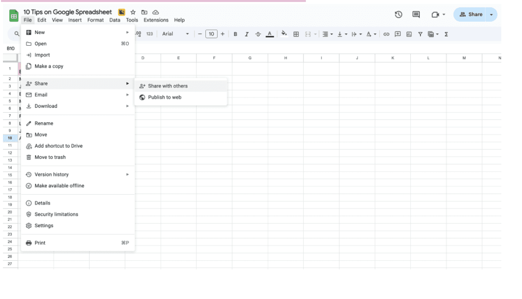
1. Click on File→Share → Share with others 

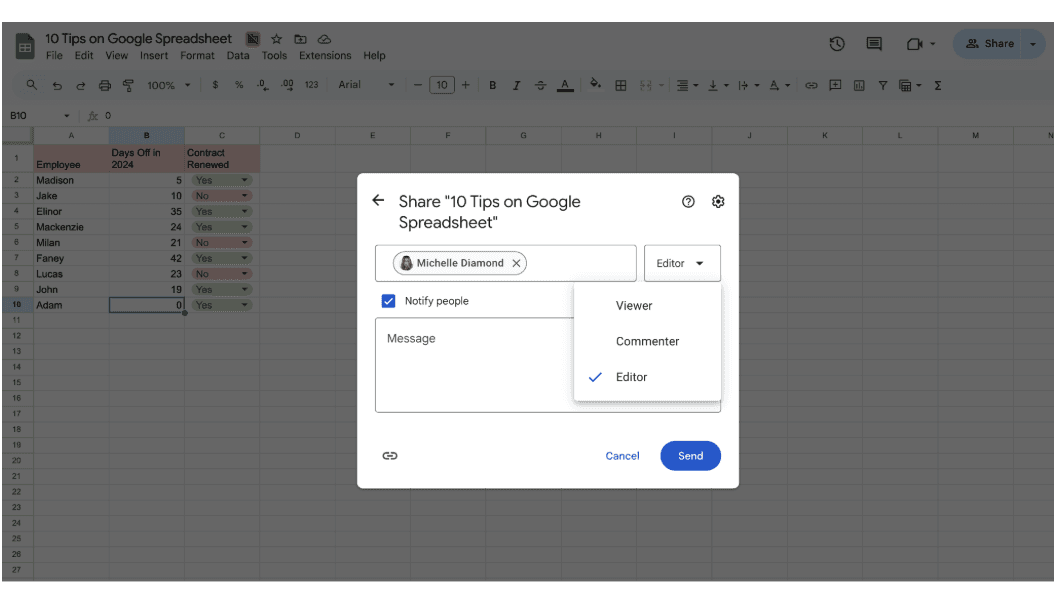
2. Select Viewer, Commenter, or Editor permissions depending on trust level.
   Next to the name, click the dropdown and select what kind of access they need,

• Viewer - Can only look at your data.

• Commenter - Can leave feedback but can’t change anything.

• Editor - Can edit the sheet (only give this to people you fully trust).

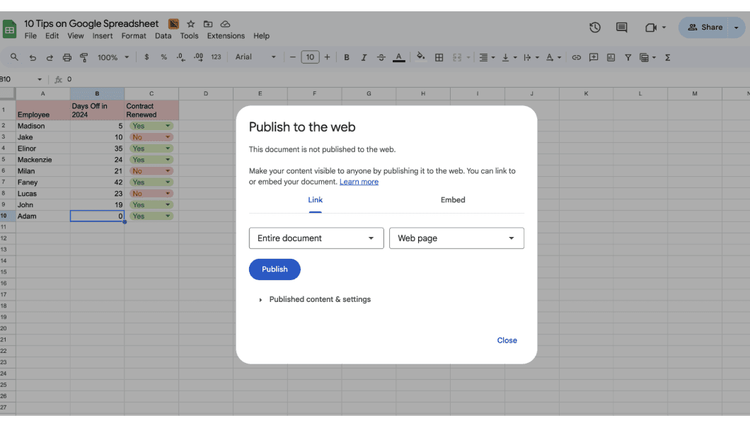
3. Pro move: Create a “read-only” version by clicking File → Share → Publish to the web. This creates a clean, read-only version that others can view but not modify. You’ll look organized and security-conscious.

2. Use Named Ranges instead of raw Cell References

We’ve all been there — staring at a long formula that looks like a secret code.

Something like =SUM(A2:A100)… and you think, “Wait, what was in column A again?”

Here’s a little trick that the smartest spreadsheet users use to make their formulas easy to read and understand — they give their data ranges names.

Let’s walk through it.

1. Click and drag to highlight the cells you usually refer to in your formulas — for example, all your numbers from B2 to B10. Then click Data and select Named Ranges.

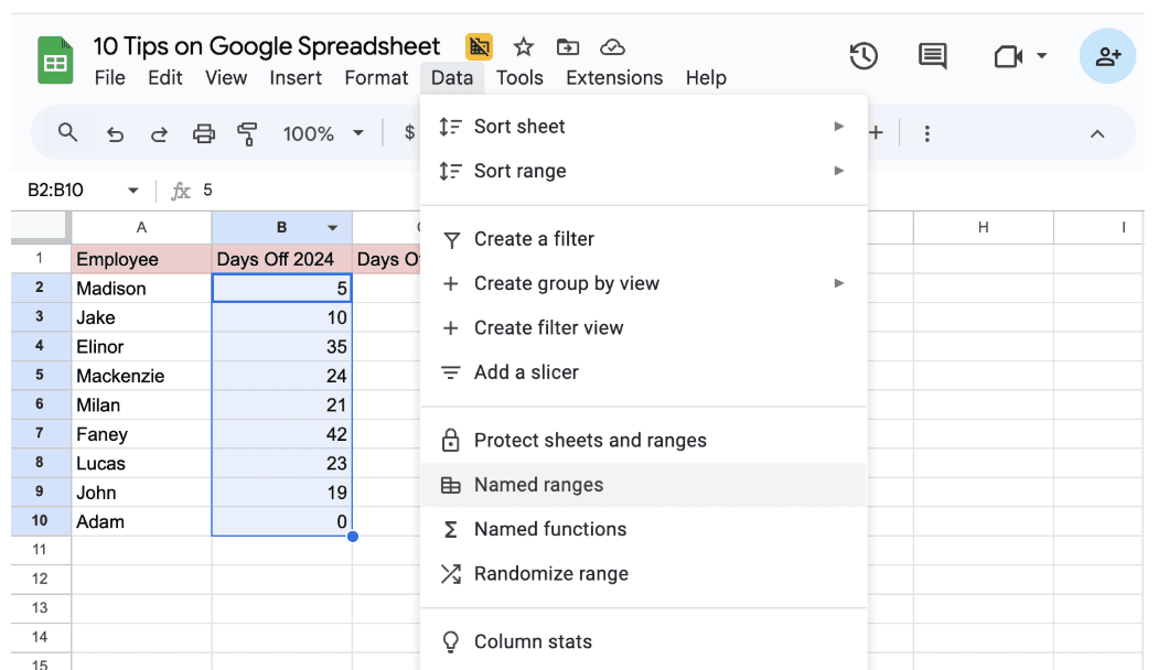
2. A side panel will appear on the right, giving it a descriptive name. And click done.

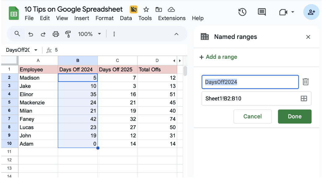
3. Instead of typing =SUM(B2:B10) just select =SUM(DaysOff2024)

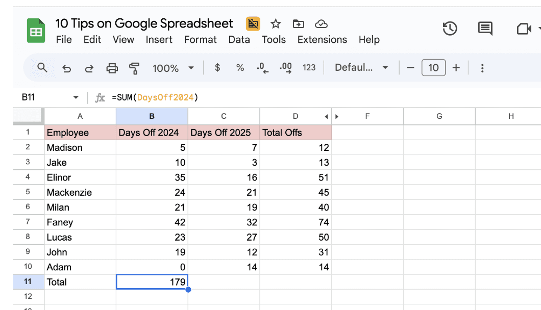
And there you have it. Your formulas are now clean, readable, and practically self-explanatory. No more decoding coordinates,  just simple, human-friendly names.

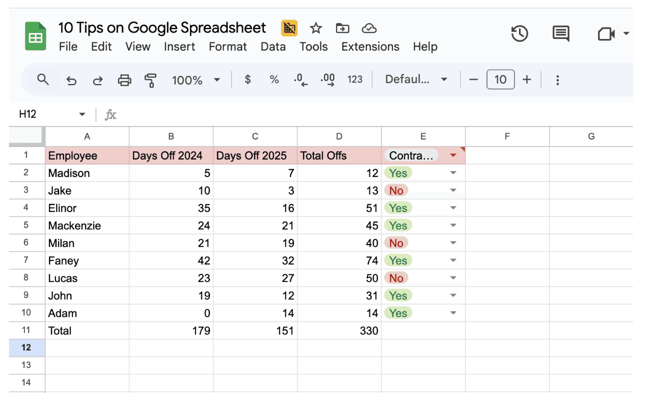
3. Use Drop-Down lists for cleaner collaboration

Your team is updating a project tracker in Google Sheets. One person types “Yes,” another writes “Y,” someone else writes “Approved,” and suddenly your filters don’t work anymore.

It’s chaos, all because of tiny typing differences.

Smart spreadsheet users solve this once and for all with drop-down lists.

Here’s how you can, too.

1. Click and drag to highlight the column or range where people should choose from predefined options — for example, your “Status” column.

Then click Data → Data validation.

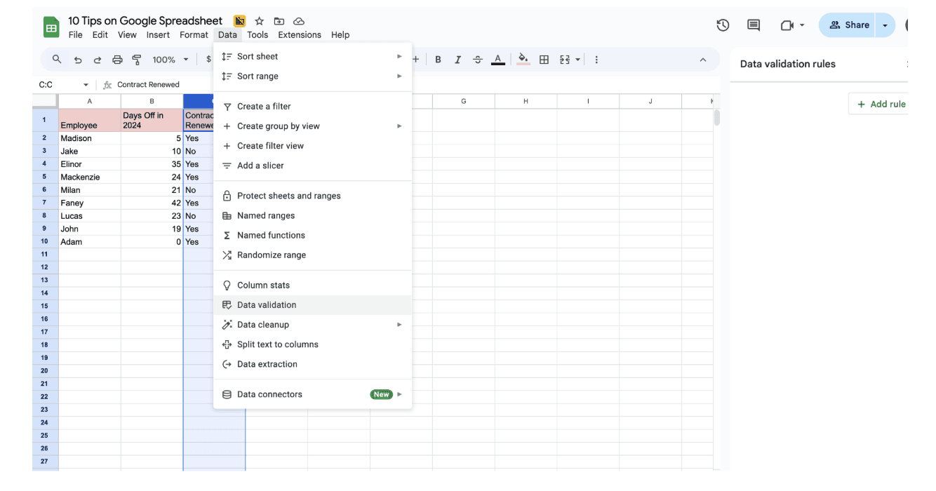
2. In the Criteria section, select Drop-down (or “List of items,” depending on your version) and click done.

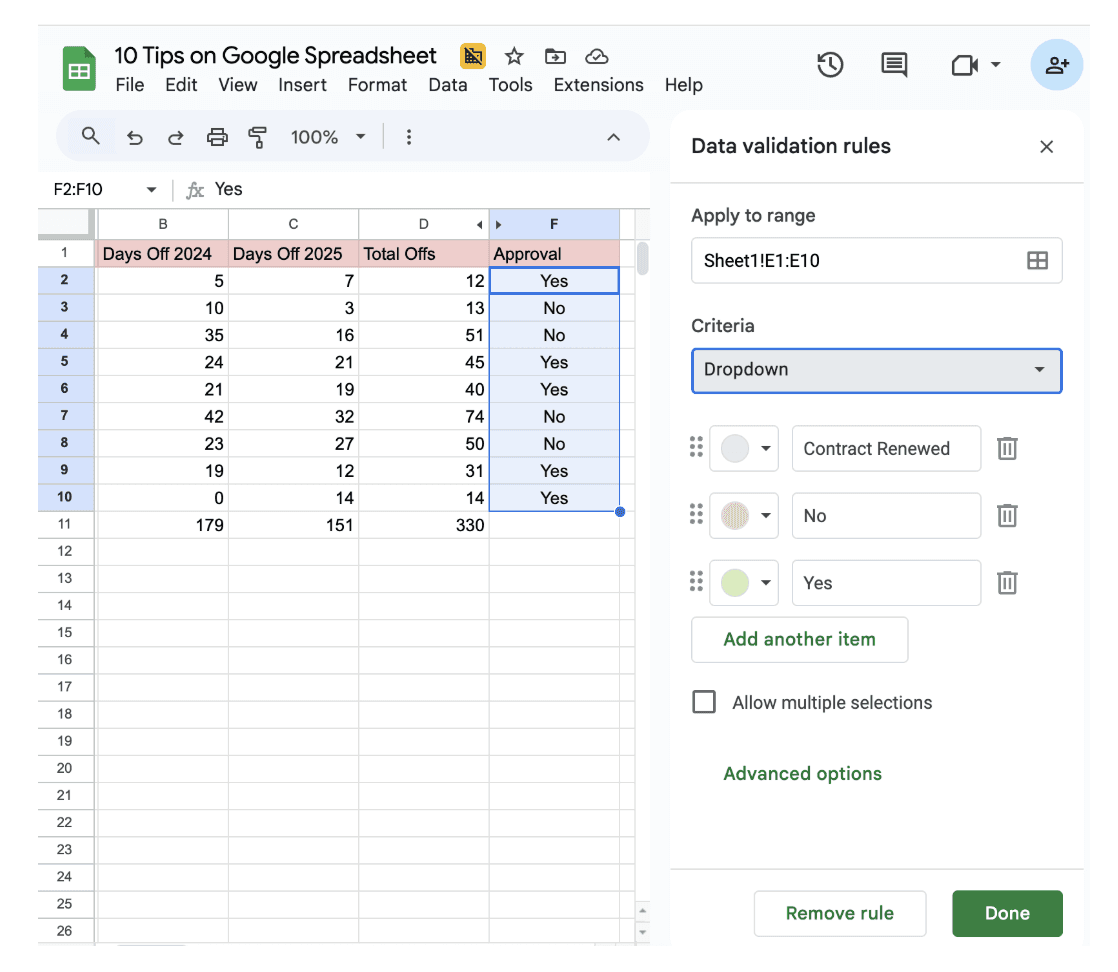
3. Instead of typing “Yes,” “yes,” “Y,” or “ok” — everyone just picks from a list. This avoids messy typos and makes your filters work like magic.

4. Conditional Formatting: let colors talk

Let’s be honest, numbers alone can be overwhelming. You scroll through rows of data, and your eyes glaze over. But then you notice something: that one spreadsheet where important values are color-coded.

Green for good, red for bad, yellow for “keep an eye on it.” It instantly makes sense.

That’s the magic of Conditional Formatting,  it makes your data speak visually.

Here’s how to set it up,

1. Click and drag over the cells that you want to format, then go to Format and select Conditional Formatting.

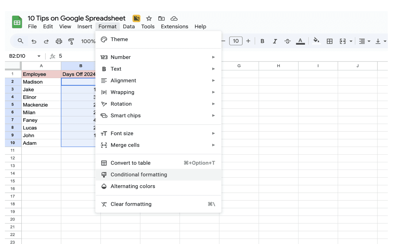
2. A side panel will appear, deciding when the color should change and click done.

For example: If the cell is greater than 15 → make it blue.

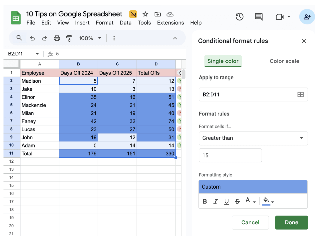
With just a few clicks, you’ve made your data visual, intuitive, and easy for anyone to understand even at a glance.

5. Protect key cells and sheets

you’ve spent hours perfecting your spreadsheet like formulas, formatting, charts, everything looks flawless. Then a well-meaning teammate tries to “help,” and suddenly half your calculations vanish. It’s nobody’s fault… but it’s a nightmare you could’ve avoided with one smart habit: protecting your key cells.

Here’s how to make sure your hard work stays untouched,

1. Go to Data and select Protect sheets and ranges.

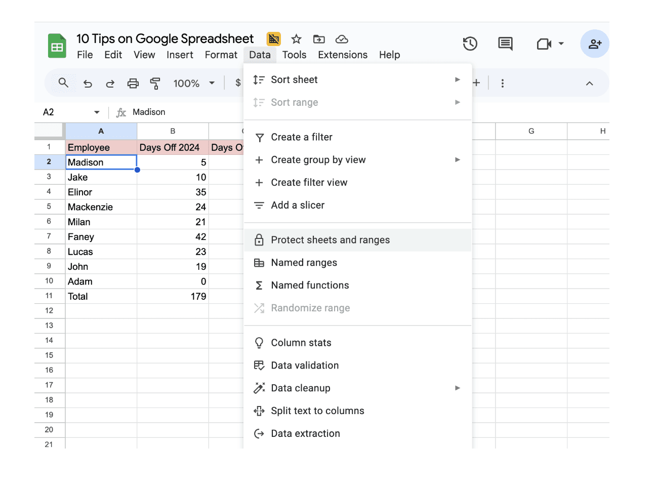
2. A panel will appear on the right side of your screen. Type a short, clear label like “Do Not Edit — Formulas” so you’ll recognize it later.

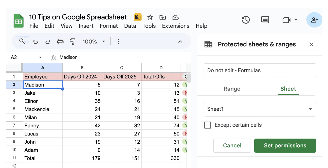
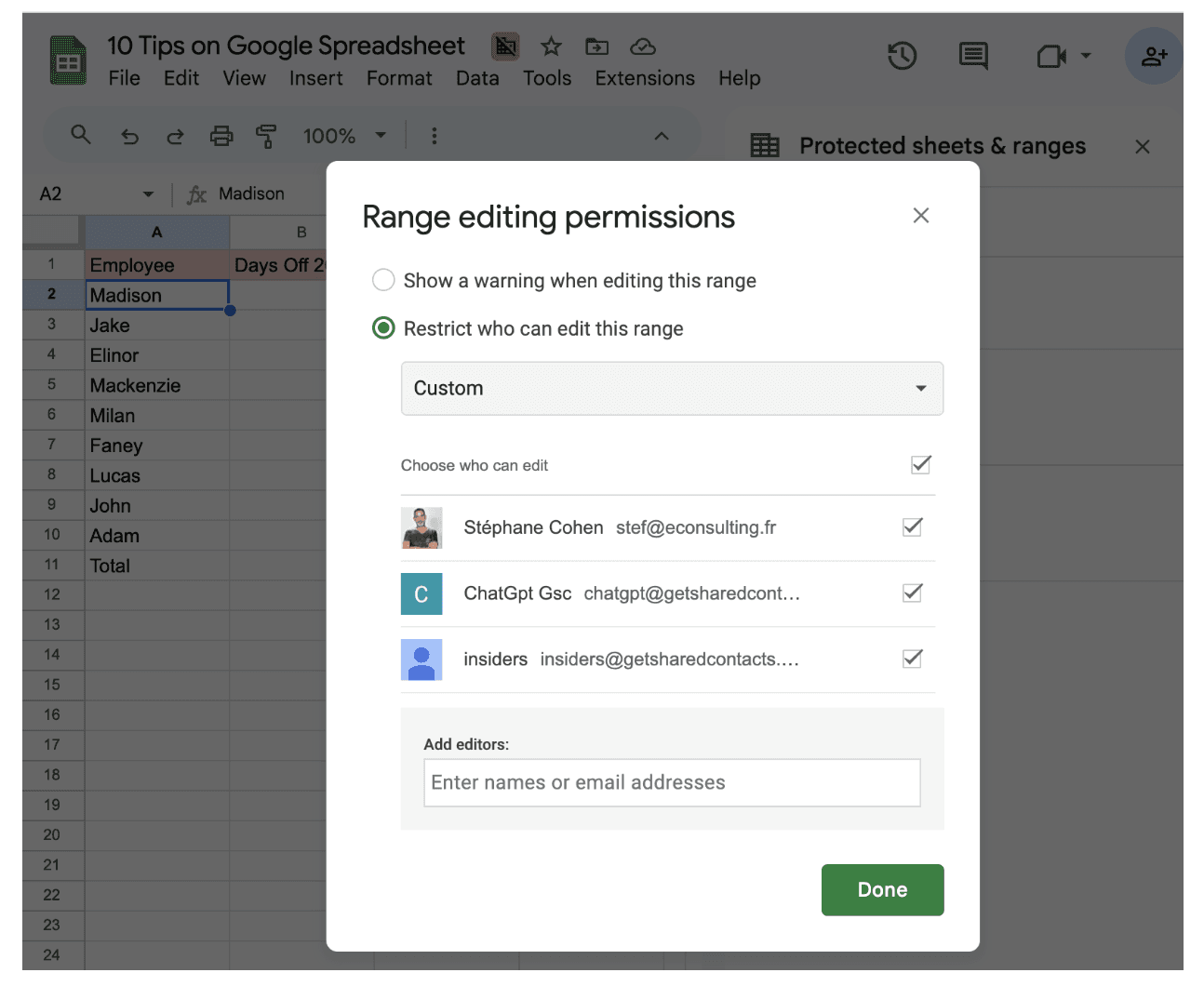
3. Click Set Permissions. Now, you get to decide who can and can’t make changes and click Done. You can:

• Allow only yourself to edit.

• Give edit rights to specific teammates.

• Or restrict everyone completely (great for final reports).

Now you can share your spreadsheet freely without worrying about accidental overwrites.

6. Use Filters and Filter Views — without messing up others’ work

You’re analyzing a shared spreadsheet with your team. You apply a filter to see only “January sales,” and suddenly someone shouts, “Hey! Where did all my rows go?”

That’s because when you use regular filters, they change the view for everyone. And in a shared sheet, that can cause serious confusion. Smart users avoid that problem completely by using Filter Views, your private filters that don’t disturb anyone else.

Here’s how you can do the same.

1. Go to Data and select Create filter view, and name it. You can privately filter data however you want.

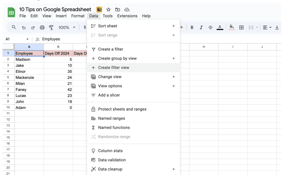
2. Now you can work on your sheet, everything you do here affects only your view, not anyone else’s.

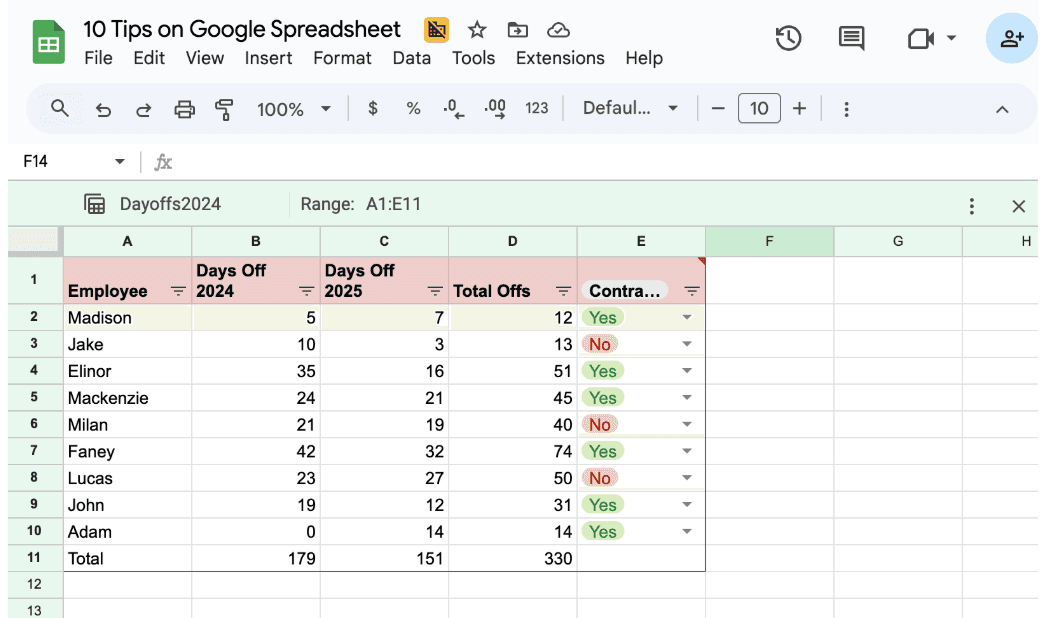
Now everyone can analyze data their own way, no more stepping on each other’s toes or losing track of what’s visible.

7. Version History — your built-in safety net

Your spreadsheet is finally perfect, and just as you’re about to close it… someone overwrites half the data. Don’t panic. Google Sheets has a hidden superpower that every smart user should know about: Version History.

Here’s how to use it.

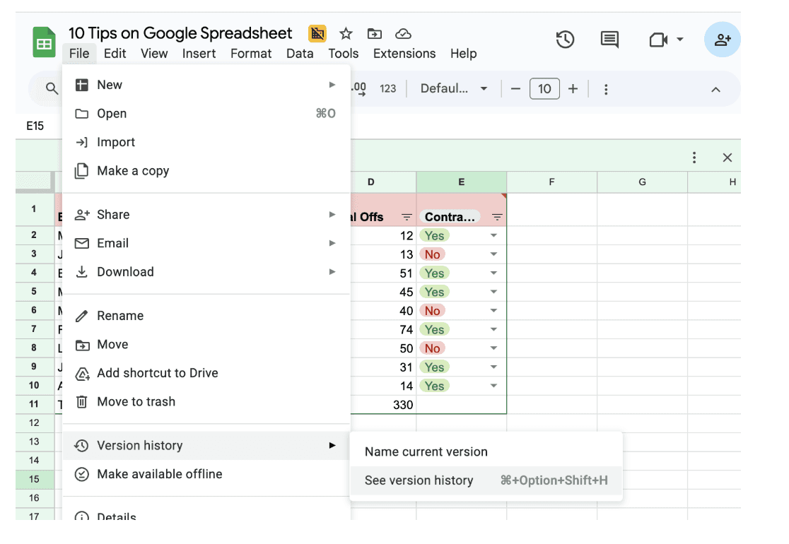
1. Click File then Version history and select See version history.

2. A panel will appear on the right side, showing all saved versions of your spreadsheet. Each one has a date, time, and the name of the person who made the edits.

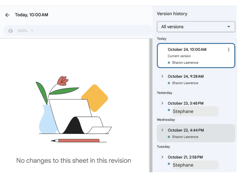
You can now experiment freely, knowing Google has your back. Every change is saved, every version recoverable.

8. Freeze Rows and Columns – to stay oriented

We’ve all been there scrolling endlessly through a big spreadsheet until you realize you have no idea which column you’re in. Was “Q3 Revenue” in column F or G? You scroll back up, lose your place, scroll down again, it’s a small but constant frustration.

To avoid that, you can Freeze rows and columns, here’s how to do,

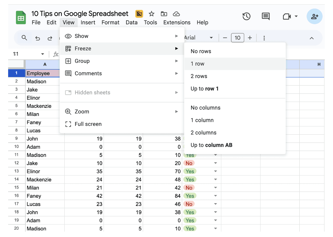
1. Select the row you want to freeze, then click View and select Freeze, and click 1 row.

2. If your spreadsheet is wide and you want to keep the first column (like names or IDs) visible, go back to View and select Freeze, and click 1 row. Now, when you scroll sideways, your first column stays put just like a label on a filing cabinet.

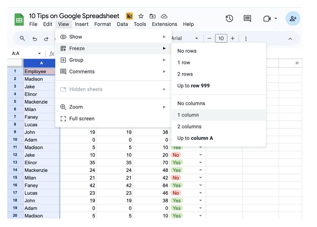
Freezing rows and columns might seem like a small trick, but it makes a huge difference in how efficiently you navigate and understand your data.

9. Use Smart fill and smart cleanup

You’ve probably noticed it before, that little gray suggestion that pops up while typing in Google Sheets, guessing what you’re about to write. That’s not luck. That’s Smart Fill, one of Google’s quietest but most powerful time-savers. Paired with Smart Cleanup, it helps you spot patterns, fix inconsistencies, and clean messy data all automatically.

Here’s how to use these built-in helpers,

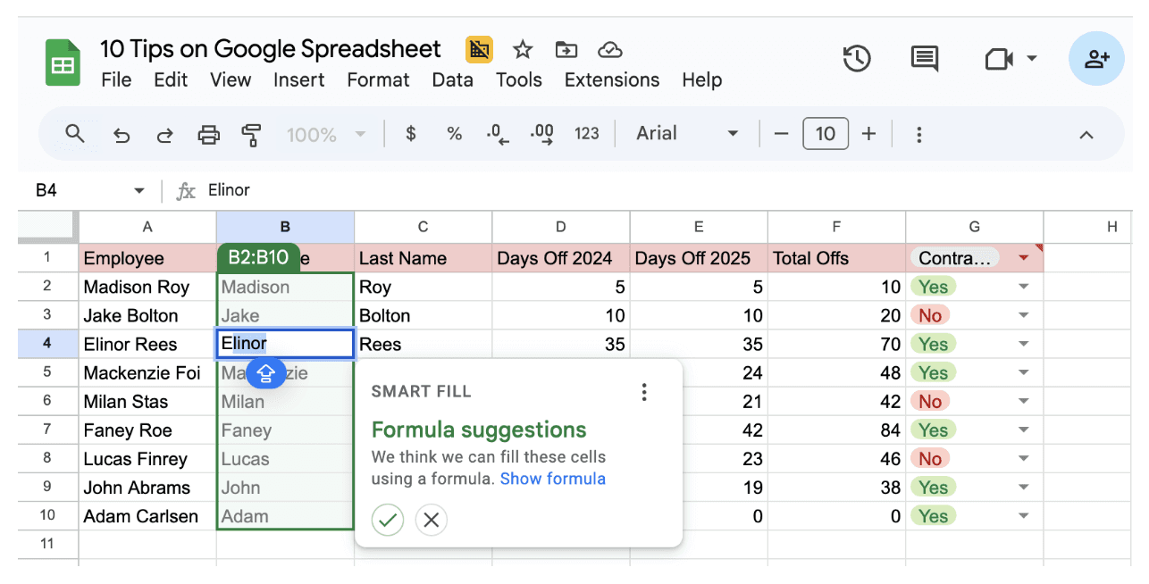
1. You have a column of full names — “John Smith,” “Lisa Brown,” and “Alex Chen” — and you want to split them into first and last names. In the next column, type “John” beside “John Smith,” and “Lisa” beside “Lisa Brown.”

When Google notices a pattern, it will show a faint preview for the rest of the column.

If the prediction looks right, just press Enter. Google Sheets will automatically fill in the rest of the column. That’s Smart Fill in action, it learns the pattern and applies it instantly.

2. Now that your data’s organized, go to Data then click Data cleanup → Cleanup suggestions. Sheets will analyze your data and show you possible improvements — like: Removing duplicate rows, fixing inconsistent capitalization, and Trimming extra spaces.

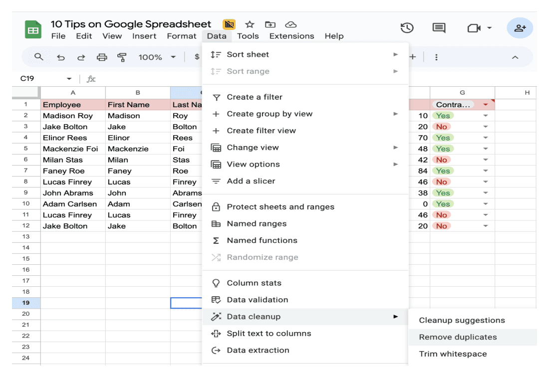
Your spreadsheet is now cleaner, more consistent, and easier to analyze.

10. Use Comments and Notes to Communicate Clearly

Ever opened a shared spreadsheet and wondered why someone changed a number or what a formula was supposed to do? That’s where smart spreadsheet users stand out: they leave breadcrumbs. Instead of sending side messages or long emails, they use comments and notes directly inside the sheet so context stays exactly where it’s needed.

Here’s how to do it,

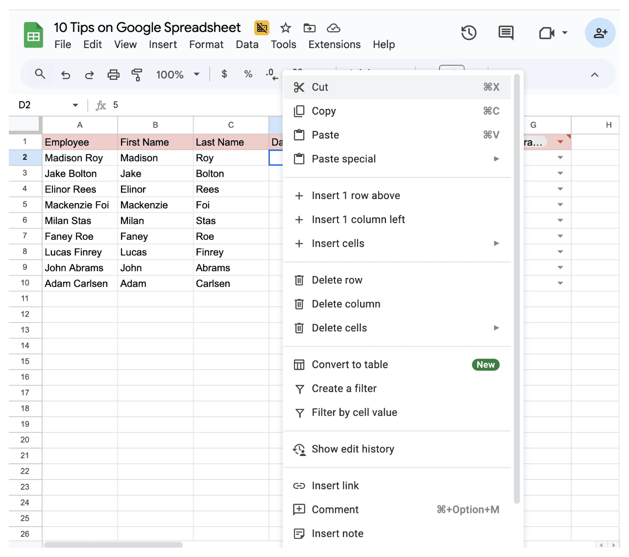
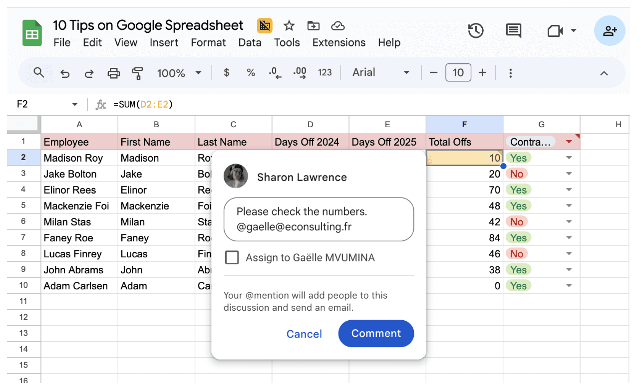
1. Right-click the cell and select Comment.

2. Type your message and you can even tag teammates by typing @theirname, and they’ll get a notification right away.

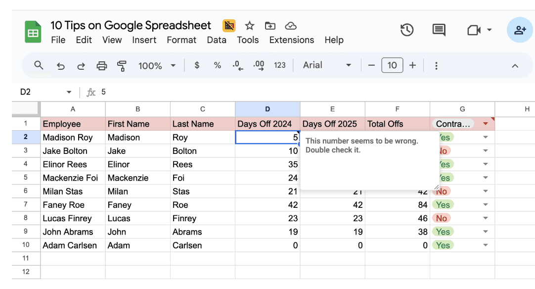
3. If you just want to leave a quiet remark (without a notification), use a Note instead. Right-click and select Insert note.

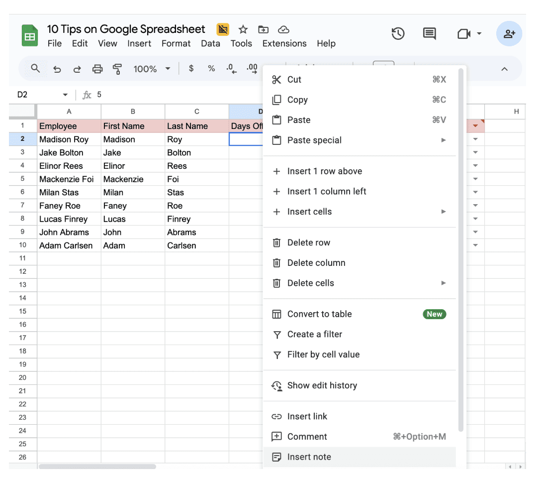
4. It will appear as a small corner marker, visible when someone hovers over the cell.

Comments keep collaboration smooth. Notes keep your work self-explanatory. Together, they make your spreadsheet feel like a living document where communication happens exactly where it should.

Smart users don’t just input data; they shape it, protect it, and make it easy for everyone else to understand. Next time you open your spreadsheet, try applying just one or two of these tips. Soon, you’ll be the calm one in the meeting, the person who makes spreadsheets look easy.

And that’s when you’ll know: you’ve leveled up from “user” to “Google Sheets pro.”